PyTorch profiling with NVIDIA Nsight Systems

Overview

This tutorial demonstrates how to profile GPU-accelerated PyTorch code with NVIDIA Nsight Systems on MeluXina GPU nodes.

To keep things simple, we profile a rather simple distributed training of a ResNet model. Using Nsight Systems, we generate a trace, analyse it in the GUI, and get an understanding of what happens when our GPU-accelerated code runs.

We also cover the main Nsight command-line options for extracting useful statistics.

Together, the presented method can help you identify why your code is not performing the way you expect it to.

1. NVIDIA profiling background

1.1. Why profiling?

When profiling, the main questions you have are

Where does the application spend time? What is each hardware component doing during that time? Am I really pushing the hardware on which I am running?

While plenty of tools exist to profile standard CPU code, they are not necessarily useful for GPU-accelerated code. The reason is that GPU execution is asynchronous. In short, CUDA API calls are issued from the CPU, after which kernels run on the GPU — but the CPU does not necessarily wait for the GPU to finish before proceeding.

This asynchrony complicates how we reason about our code performance compared to standard CPU code.

1.2. Understanding the differences between Nsight Systems and Nsight Compute

Profiling GPU code requires specialized tools; NVIDIA provides two complementary profilers for this purpose.

Nsight Systems provides a system-wide timeline and answers questions such as:

• When is the GPU working or idle?
• Is the CPU preparing data while the GPU computes?
• Are multiple DDP ranks progressing together?
• What surrounds a phase with low GPU usage?
• What are the most frequent CUDA API calls?
• What are the most time-consuming kernels?

Nsight Compute is a kernel-level profiler. After Nsight Systems identifies an expensive CUDA kernel, Nsight Compute can be used to investigate why that kernel is slow using metrics such as occupancy, memory bandwidth, cache behavior, and warp stalls.

Rule of thumb: start with Nsight Systems to identify the main bottlenecks in your code. Then, focus on one/a few problematic kernel(s) and use Nsight Compute for a deeper analysis.

Important This tutorial focuses on Nsight Systems. For more information on Nsight compute, see this link. Unfortunately, Nsight Compute cannot work with the output of NSight Systems (which is an .nsys-rep file). We have to perform a separate run with Nsight compute.

2. Profiling a PyTorch job with Nsight Systems

In this section, we run and profile a simple PyTorch training script. The script uses a single MeluXina GPU node and its 4 GPUs.

To do this, we need two files:

• a Python script containing the training loop resnet_profile.py
• a Slurm submission script nsys_profile.sh

Both scripts are available in this repository. We recommend creating a separate working directory (with sufficient free space and inodes) on Meluxina and copying the files there.

2.1 The Python script to profile

You will see in the Python code several calls to nvtx_range. NVTX ranges are used to annotate important stages of the training loop, for example:

def run_epoch(self, epoch):
    ...
    with nvtx_range("Forward pass"):
        output = self.model(source)

    with nvtx_range("Loss computation"):
        loss = F.cross_entropy(output, targets)
    ....

Each nvtx marks a region of the training loop (a step, an epoch, the forward pass, and so on).

Once the trace is post-processed and opened in the Nsight Systems GUI, these markers appear as NVTX ranges on the timeline (see NVTX rows). They tell you exactly which part of the code was running at any given moment.

This makes it easy to understand the "mechanics" of the profiled code. For instance, you can see when source, targets = next(data_iterator) runs and how long it takes.

Skipping the first epochs

This is specific to AI training. If the code your want to profile is not an AI training, this is not relevant.

Training performance is often unstable at the beginning of a run, so the initial warm-up epochs are usually excluded from measurement. These early epochs incur one-time costs such as CUDA initialization, memory allocation, kernel autotuning, DataLoader startup, and compilation overhead. Profiling should therefore begin only once throughput has stabilized.

2.2 The Slurm script

The repository contains a complete example Slurm submission script named nsys_profile.sh

Submit the job with:

sbatch --account=p2xxxxx nsys_profile.sh

where p2xxxxx is your project identifier.

It is very interesting to pay attention to the command structure that we use to run the profiling:

srun [Slurm options] nsys profile [Nsight options] application [application options]

Technical note - profiling only what matters

Sometimes, you do not want to profile a script's entire runtime. For instance, you may not care about its first lines, where modules are typically loaded. On top of this, Nsight Systems does not officially support runs longer than 5 minutes, see the official NSight documentation.

We tell Nsight Systems to profile only part of the code with:

--capture-range=cudaProfilerApi
--capture-range-end=stop

We recommend to use torch.cuda.profiler.start() and torch.cuda.profiler.stop() around the region of interest of the python code. This allows you to control what you want to profile. In the case of a model training for instance, you want to avoid profiling python module imports, model setup and initialization. You are just interested in the training loop.

To only capture what you need to, you could adopt such a structure to have a more precise control on what you profile:

import torch
import myothermodule
# Imports and application initialization

# Model creation, dataset loading, warm-up, etc.

torch.cuda.profiler.start()

# Training loop or computation phase of interest
for epoch in range(num_epochs):
train_one_epoch()

torch.cuda.profiler.stop()

# Checkpoint saving, evaluation, cleanup, and other code

3. Nsight report files

After the job completes, the output directory contains a report such as:

${TIMESTAMP}_nsys_resnet_output/
└── resnet_profile.nsys-rep

Depending on the options and Nsight Systems version, an SQLite export or temporary .qdstrm file may also appear. The .nsys-rep file is the report we will use to analyse the runtime with the GUI but also with command-line analysis tools.

Let's start with the visual interpretation of the profiling.

4. Analysing an .nsys-rep report with the GUI

Install the Nsight Systems graphical interface locally or use an appropriate graphical connection to MeluXina. Download the .nsys-rep file when using a local installation.

4.1 Interacting with the timeline

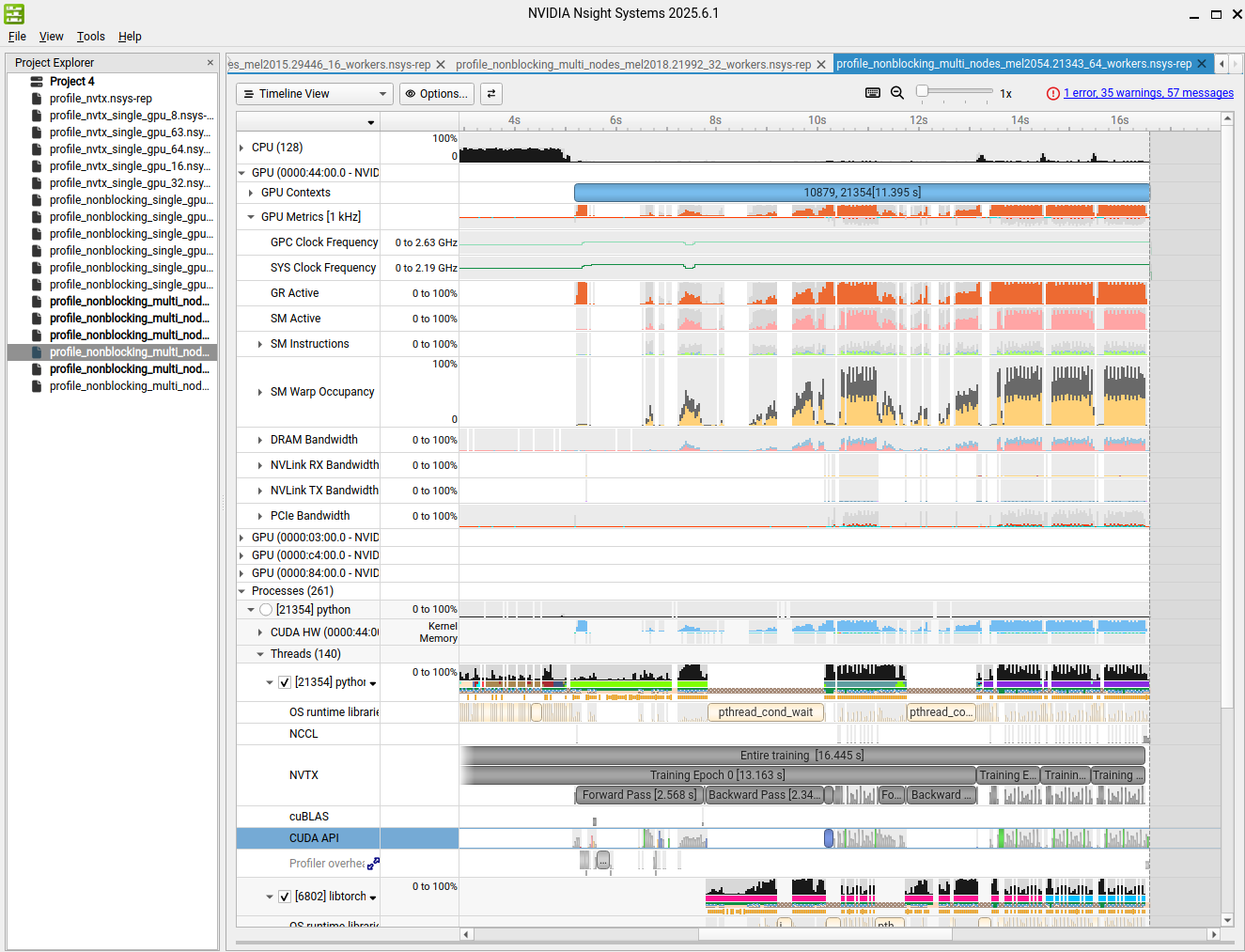
A useful inspection strategy is to first locate GPU idle regions, then identify the surrounding NVTX ranges, and finally inspect memory transfers, CPU activity, and communication that occur during the same period. You can do this quite easily by selecting a part of the timeline. Select the starting point of your region of interest, keep the left button press and slide to the end of the period you are interested in. You then have the possibility to filter and zoom-in (right click to see those options).

Once your period of interest is selected, you can then have a closer look at:

• NVTX
• CUDA HW
• kernels
• memory copies
• GPU metrics, if collected
• relevant CPU and OS runtime tracks.

4.2 NVTX rows

As mentione before, when you have the possibility to add nvtx context managers, you can have a better understanding of what part of your code triggered some hardware usage /API calls.

For example, we select below a region where the GPU usage (orange curve) has a gap.

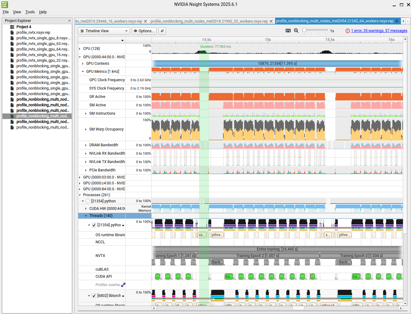
We can see here that the gap in the GPU utilization are happenning periodically at the beginning of each epoch. It would have been difficult to guess this without the nvtx ranges !

4.3 CPU activity

CPU tracks show when processes and threads run or block. In PyTorch training, inspect:

• DDP training processes (the Processes containing the CUDA HW row, there is one per GPU);
• CUDA runtime calls;
• OS runtime waits;
• NCCL-related activity.

A busy CPU does not guarantee a busy GPU — it can be the opposite. Your CPU might be working to produce data the GPU will need, while the GPU sits idle. Also, be careful with oversuscrbibing with too many workers. It can give you an impression that "nothing is happenning nor on the CPU or the GPU".

4.4 GPU activity

The CUDA HW row shows, for each GPU, when the GPU is actually executing work; the GPU kernels row breaks this down into individual kernel launches. When these rows are packed with closely spaced colored blocks, the GPU is busy. Gaps between the colored blocks are what people call GPU gaps or starvation: the GPU is idle while something else on the system catches up.

Not every gap matters. Some gaps are difficult to avoid and can be a one-time thing (context creation, first memory allocation, kernel autotuning, DataLoader warm-up) and can be ignored. Tiny gaps between kernels are often just launch latency. The question that matters is: does the gap recur often enough, and last long enough, to measurably reduce throughput? A gap that recurs once per training step and costs a few milliseconds is far more important than a one-off gap at startup. Zoom in and measure the interval before interpreting it (see Interacting with the timeline).

Classify a gap by what else happens at the same instant. The cause is rarely visible on the GPU rows alone. Keep the time axis aligned across tracks and ask, "what is active while the GPU is idle?". This can be tricky, but it is also where you will find the changes that yield substantial performance improvements. Below, we list the main culprits for such gaps:

If, during the gap, you see…	…the gap is most likely caused by
an active DataLoader next NVTX range, with CPU threads busy in preprocessing	the input pipeline not producing batches fast enough. The GPU is therefore waiting for the batches to be ready
a cudaStreamSynchronize, cudaDeviceSynchronize, or .item() call on the CPU, followed by idle	a blocking synchronization that forces the CPU to wait for the GPU
NCCL collective kernels (e.g. all-reduce) that have not started, or another rank still computing	distributed communication, or a straggler rank (see DDP and stragglers)
a large host-to-device copy still running, especially from pageable (unpinned) memory	data transfer between the host (the CPU) and the device, which starves the following kernels of work
an epoch or iterator NVTX boundary (end of one epoch, start of the next)	epoch-boundary overhead: sampler reshuffle, DataLoader re-creation

Only once you have correlated the idle interval with the activity around it should you decide what to change — and even then, treat that correlation as a hypothesis to test rather than a conclusion.

4.5 Uneven rank performance in PyTorch DDP

This example uses PyTorch DistributedDataParallel (DDP) to distribute training across GPUs. Each DDP rank uses one GPU and typically owns its own DataLoader.

Because the ranks must synchronize frequently, they cannot progress independently. During gradient synchronization, for example, every rank must wait until the slowest rank arrives before the collective operation can complete.

As a result, an imbalance in the workload — where a single rank does more work or runs slower than the others — reduces utilization across all GPUs. Such a slow or blocking rank is called a straggler, and the resulting slowdown is known as the straggler effect.

Whenever possible, compare the timelines of all four ranks rather than inspecting a single GPU: a straggler only becomes visible when the ranks are viewed side by side.

5. Command-line analysis

As you have seen, the timeline of Nsight can look quite heavy and it might be hard to understand what is affecting performances. It is possible to get runtime information as text and numbers from the CLI, plus more advanced diagnostics.

Load Nsight Systems in an interactive allocation:

salloc -A p2xxxxx -p gpu --qos=default -N 1 -t 02:00:00
module load Nsight-Systems

The main commands are:

nsys stats    -> generate statistical summaries
nsys analyze  -> apply available diagnostic rules

Both are also available in the Nsight Systems UI: switch from Timeline View (top left) to Diagnostics Summary for nsys analyze, or right-click an activity row and choose Show in Events View for nsys stats.

Check the locally installed version for available reports and rules:

nsys stats --help-reports
nsys analyze --help

5.1 nsys analyze

nsys analyze report.nsys-rep applies diagnostic rules that can point to symptoms such as pageable asynchronous copies, synchronization, or long GPU idle gaps.

For example, an analyzer may suggest using pinned memory instead of pageable memory.

Use this information and go back to the visual timeline to determine whether an activity delays subsequent GPU work or overlaps with other activity.

We already discussed gpu gaps. nsys analyze also gives some hints on the ones strongly affecting performance. Once again, use this information in complement to the timeline and try to understand what is the underlying issue. Usually, inspecting the following points help you understand what is the culprit(s):

• the surrounding NVTX range;
• DataLoader activity;
• CPU blocked or active state;
• H2D copies;
• synchronization and communication;
• whether the gap occurs at startup, between steps, or between epochs.

5.2 nsys stats

Where the GUI shows a timeline, nsys stats prints the same information as tables of numbers. This is convenient inside a script, or whenever you only need a few figures rather than a full visual inspection. Each table is called a report, and you request one or more of them with --report.

Start by listing the reports your installed version provides:

nsys stats --help-reports

Most reports come in two flavours: a raw form (for example cuda_gpu_kern_sum) and a …_pretty form that prints human-readable units such as ms, us, and KB. The pretty variants are easier to read; the raw ones are handy when you want to post-process the numbers. A typical call collects the four reports we use most:

nsys stats \
    --report nvtx_pretty,cuda_api_pretty,cuda_gpu_kern_pretty,cuda_gpu_mem_time_pretty \
    report.nsys-rep

You can narrow or reorganise a report with a few options:

• --stats count,total,min,max,avg limits the columns that are printed;
• --group name (or demangled, stream_id, …) changes how the rows are grouped;
• --sort orders the rows, usually so the most expensive entries appear first.

NVTX summary (nvtx_pretty)

The NVTX summary compares your annotated regions by count and by total, average, median, minimum, and maximum duration. It is a numerical alternative to the UI timeline for spotting long epochs, steps, or DataLoader next waits (see NVTX rows). Note, though, that this report is empty unless your code was annotated with NVTX — for instance when the source is not modifiable, such as code running inside a container you do not control.

Read it as a first triage: an epoch or step whose average is far above its median, or whose maximum is much larger than its average, points to irregularity worth inspecting on the timeline. Because the ranges mirror your code structure, the summary also tells you where the time goes — the forward pass, the backward pass, or data loading.

CUDA API summary (cuda_api_pretty)

The CUDA API summary groups the runtime and driver calls by name and reports how often each is called and how much time it accounts for. It answers two different questions: which calls are the most frequent, and which are the most time-consuming.

A training loop dominated by a very high count of small calls (for example many cudaLaunchKernel or cudaMemcpyAsync) suggests launch overhead, whereas a few very expensive calls (for example cudaMalloc or a synchronising call) point elsewhere. Compare this view with the timeline to decide whether the calls overlap with GPU work or block it (see CPU activity).

GPU kernel summary (cuda_gpu_kern_pretty)

The GPU kernel summary lists the kernels that actually ran on the device, with their count and total, average, minimum, and maximum duration, and usually their share of GPU time. This is where you identify the most expensive kernels — the ones Nsight Systems flags as worth a closer look (see GPU activity).

If a single kernel dominates the total, it is the natural first target for the deeper, kernel-level analysis that Nsight Compute provides. Recall that Nsight Compute is a separate, targeted collection: it does not read the .nsys-rep file (see Understanding the differences between Nsight Systems and Nsight Compute).

Memory-operation summaries (cuda_gpu_mem_time_pretty)

Memory summaries describe the copies between host (H) and device (D) : H2D, D2H, and D2D (device-to-device), with their type, count, duration, and volume. If H2D copies dominate memory-operation time, investigate them on the timeline.

Do not confuse:

percentage of memory-operation time

with:

percentage of total application time

H2D may dominate memory-operation time but still be only a small part of the full training step. It is a bottleneck only when it aligns with GPU idle time.

6. Conclusion

Throughout this tutorial we have profiled a single example — the distributed training of a ResNet model — but the method carries over to any GPU-accelerated application. Nsight Systems never tells you directly "your code is slow". Instead, it shows you what the hardware is doing, and your job is to translate those observations into an understanding of how your application behaves and how its implementation affects runtime performance. A few general principles help:

• Start wide, then zoom in. Begin with the system-wide timeline to locate the interesting regions — where the GPU is idle, where a phase is unusually long — and only then zoom into the calls inside them. Do not start by interpreting individual events before you know where you are.
• Map the timeline to your code. Annotate the important regions with NVTX when you can do it, so that every gap or spike carries the name of the code that produced it. Without that mapping you are reading hardware activity without knowing which part of your program it corresponds to, which is more delicate.
• Ask "what else is happening at the same time?". A GPU gap on its own means little. The cause becomes clear only when you keep the time axis aligned across tracks and see what is active — a DataLoader, a copy, a synchronization, another rank — while the GPU waits.
• Combine the GUI and the command line. Use the timeline to see when and why something happens, and nsys stats and nsys analyze to confirm it with numbers and to catch symptoms you might otherwise miss.

The goal is not to eliminate every small gap — many are harmless startup cost or launch latency — but to find the recurring inefficiency that actually limits throughput, understand its cause, and verify that fixing it helps.