An example of performance comparison between pandas and cudf
Introduction
In this short tutorial, we assume that we have performed a profiling of a python code involving large datasets and identified the bottleneck. We then extracted the corresponding code in a function called sample_data that you can find below:
def sample_data(dfg):
    return dfg.groupby(["Gid"]) .apply( lambda x: x.sample( x["Nb"].iat[0], weights=x["Prob"], random_state=1, replace=True)) .reset_index(drop=True)
Our goal here is to try to come up with a more efficient solution.
The Methods in Focus
-
Default Pandas Implementation (
sample_data): This method uses standard Pandas operations. It's straightforward and represents the typical approach many Python developers might initially consider. -
Alternative Pure Pandas Implementation (
sample_data_v2): This version also relies on Pandas but employs a different logic. This function has been found by asking Chat-GPT to optimizesample_datajust to see if it can lead to better performances. -
Numba Implementation (
sample_data_numba): By incorporating Numba, a Just-In-Time compiler, we aim to speed up the operation. Numba is known for its ability to optimize numerical computations, which could be a game-changer for data sampling tasks. But let's see if this works in the present case. -
CuDF Implementation (
sample_data_cudf): This method uses CuDF, a GPU-accelerated DataFrame library. It's designed to leverage the parallel computing power of GPUs, offering potential speedups for large-scale data operations.
Preliminary imports
In order to use cuDF we will need to work on the GPU partition and import the appropriate modules. Whether you use an interactive session (salloc -A [YOUR ACCOUNT] -p gpu --qos default -N 1 -t 8:00:0) or a batch script, you should source the following script before launching the python code we will give below.
#!/bin/bash -l
module --force purge
ml env/release/2023.1
ml Python/3.10.8-GCCcore-12.3.0
ml cuDF
Code for the different functions
import pandas as pd
import numpy as np
import random
import numba
import cudf

def sample_data(dfg):
    return dfg.groupby(["Gid"]) .apply( lambda x: x.sample( x["Nb"].iat[0], weights=x["Prob"], random_state=1, replace=True)) .reset_index(drop=True)

def sample_data_cudf(dfg):
    return cudf.DataFrame.from_pandas(dfg).groupby(["Gid"]).apply( lambda x: x.sample( x["Nb"].iloc[0], weights=x["Prob"], replace=True)) .reset_index(drop=True)

def sample_data_v2(dfg):
    # Generate a sequence of indices for sampling
    indices = dfg.groupby('Gid').apply(lambda x: pd.Series(x.index).sample(n=x['Nb'].iat[0], weights=x['Prob'], random_state=1, replace=True))

    # Flatten the indices series and use it to index into the original DataFrame
    return dfg.loc[indices.values].reset_index(drop=True)

@numba.jit(nopython=True)
def numba_sampling(gid, nb, prob, size):
    result_indices = np.zeros(size, dtype=np.int64)
    unique_gid = np.unique(gid)

    start_idx = 0
    for g in unique_gid:
        mask = gid == g
        count = nb[mask][0]
        weights = prob[mask]
        a = np.where(mask)[0]
        # selected_indices = np.random.choice(a = a, size=count, replace=True, p=weights)
        selected_indices = np.random.choice(a = a, size=count, replace=True)
        result_indices[start_idx:start_idx+count] = selected_indices
        start_idx += count

    return result_indices

def sample_data_numba(dfg):
    gid_array = dfg['Gid'].values
    nb_array = dfg['Nb'].values
    prob_array = dfg['Prob'].values

    total_size = dfg.groupby('Gid')['Nb'].first().sum()
    selected_indices = numba_sampling(gid_array, nb_array, prob_array, total_size)

    return dfg.iloc[selected_indices].reset_index(drop=True)
Experimentation
Below we provide the full python script along with some explanations.
Click to expand!
# Copyright 2021-2024 Luxembourg National SuperComputer (MeluXina)
# @LuxProvide
# Marco Magliulo, Wahid MAINASSARA
import pandas as pd
import numpy as np
import random
import time
import numba
import cudf
def remove_outliers_trim(data, trim_percentage):
# Sort the data
sorted_data = np.sort(data)
# Compute the number of data points to trim
trim_count = int(len(sorted_data) * trim_percentage / 100)
# Remove the outliers from both ends
trimmed_data = sorted_data[trim_count:-trim_count]
# Compute the average of the trimmed data
trimmed_avg = np.mean(trimmed_data)
return trimmed_avg
def time_function(func):
def wrapper(*args, **kwargs):
runtimes = []
for _ in range(10):
start_time = time.time()
func(*args, **kwargs)
end_time = time.time()
runtime = end_time - start_time
runtimes.append(runtime)
min_runtime = min(runtimes)
max_runtime = max(runtimes)
avg_runtime = sum(runtimes) / len(runtimes)
treshold = 10
trimmed_avg = remove_outliers_trim(runtimes, treshold)
print("This is the list of all runtimes")
print(runtimes)
print(f"Minimum Runtime: {min_runtime:.6f} seconds")
print(f"Maximum Runtime: {max_runtime:.6f} seconds")
print(f"Average Runtime: {avg_runtime:.6f} seconds")
print(f"Trimmed average runtime ({treshold} percentile removed): {trimmed_avg:.6f} seconds")
# Store trimmed_avg in the function attribute
# this is useful to recover the run time afterwards
wrapper.trimmed_avg = trimmed_avg
return wrapper
@time_function
def sample_data(dfg):
return dfg.groupby(["Gid"]) .apply( lambda x: x.sample( x["Nb"].iat[0], weights=x["Prob"], random_state=1, replace=True)) .reset_index(drop=True)
@time_function
def sample_data_cudf(dfg):
return cudf.DataFrame.from_pandas(dfg).groupby(["Gid"]).apply( lambda x: x.sample( x["Nb"].iloc[0], weights=x["Prob"], replace=True)) .reset_index(drop=True)
@time_function
def sample_data_v2(dfg):
# Generate a sequence of indices for sampling
indices = dfg.groupby('Gid').apply(lambda x: pd.Series(x.index).sample(n=x['Nb'].iat[0], weights=x['Prob'], random_state=1, replace=True))
# Flatten the indices series and use it to index into the original DataFrame
return dfg.loc[indices.values].reset_index(drop=True)
@numba.jit(nopython=True)
def numba_sampling(gid, nb, prob, size):
result_indices = np.zeros(size, dtype=np.int64)
unique_gid = np.unique(gid)
start_idx = 0
for g in unique_gid:
mask = gid == g
count = nb[mask][0]
weights = prob[mask]
a = np.where(mask)[0]
# selected_indices = np.random.choice(a = a, size=count, replace=True, p=weights)
selected_indices = np.random.choice(a = a, size=count, replace=True)
result_indices[start_idx:start_idx+count] = selected_indices
start_idx += count
return result_indices
@time_function
def sample_data_numba(dfg):
gid_array = dfg['Gid'].values
nb_array = dfg['Nb'].values
prob_array = dfg['Prob'].values
total_size = dfg.groupby('Gid')['Nb'].first().sum()
selected_indices = numba_sampling(gid_array, nb_array, prob_array, total_size)
return dfg.iloc[selected_indices].reset_index(drop=True)
def test_sample_data(nValues):
# create a sample dataframe for testing
randomGID= [random.choice([1,2]) for _ in range(nValues)]
randomNb= [random.choice([1,2,3]) for _ in range(nValues)]
randomProb = [random.uniform(0, 1) for _ in range(nValues)]
data = {
"Gid": randomGID,
"Nb": randomNb,
"Prob": randomProb
}
dfg = pd.DataFrame(data)
print("Testing original implementation")
sample_data(dfg)
print("\n")
print("Testing pure python v2 implementation")
sample_data_v2(dfg)
print("\n")
print("Testing numba implementation")
sample_data_numba(dfg)
print("\n")
print("Testing cudf implementation")
sample_data_cudf(dfg)
return sample_data.trimmed_avg, sample_data_v2.trimmed_avg, sample_data_numba.trimmed_avg, sample_data_cudf.trimmed_avg
if __name__ == '__main__':
start_value = 10000
end_value = 10000000
nTests = 10
# nrows contains the list of the number of rows that will tests one after the other
nrows = np.linspace(start_value, end_value, num=nTests).astype(int)
y = []
for nrowsi in nrows:
# we will test for a number of lines in the dataframe xi the different implementations and collect the trimmed average runtime
y.append(test_sample_data(nrowsi))
import matplotlib.pyplot as plt
# Unzip the tuples in y
y1, y2, y3, y4 = zip(*y)
# Create the plot
plt.plot(nrows, y1, label='Default implementation')
plt.plot(nrows, y2, label='Alternative pure pandas implementation')
plt.plot(nrows, y3, label='Numba implementation')
plt.plot(nrows, y4, label='Cudf implementation')
# Add labels and legend
plt.xlabel('Number of rows in the df')
plt.ylabel('Trimmed average time in seconds')
plt.title('Comparison of different implementations for the sampling function')
plt.legend()
plt.draw()
# Save the plot as a PDF
plt.savefig('plot.png')
The performance of each function is tested using a decorator, time_function, which captures runtime statistics such as minimum, maximum, average, and trimmed average runtimes. This decorator will allow us to have an idea of how the different functions perform. Also, as the following lines are showing, we run each function 10 times to have a reasonnable estimate of their runtime.
def time_function(func):
    def wrapper(*args, **kwargs):
        runtimes = []
        for _ in range(10):
            [...]
wrapper.trimmed_avg = trimmed_avg. What we do here is that we capture the trimmed average of the different runtimes. Indeed, the first time the code reaches the function based on numba and the one based on cudf are much slower than the successive runs. In order to remove those slower runs, we get rid of the outliers.
Info: The observed slowdown in the first run of a function accelerated by Numba, a just-in-time (JIT) compiler for Python, is primarily due to the compilation process that takes place during the initial execution. . Info: cuDF is a Python GPU DataFrame library for manipulating data using an API. When you first use cuDF in your application, several things happen like loading the CUDA toolkit, allocating the memory and the GPU and compiling CUDA kernels if needed. This is why the initialization and warm-up phase can take significant time.
Effect of the dataframe size
We conduct our experiments using a function, test_sample_data, that generates a DataFrame with a varying number of rows, simulating different data scales. This is to have some insights on how each function scales and performs under varying loads. Here, we test 10 different number of rows equally spread between 1000 and 10000000 rows. Feel free to change it in case you want to test the code!
Insights and Analysis
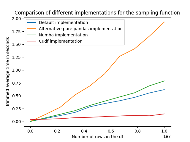
The below figures summarizes the effect of the dataframe size on the trimmed average runtime of the four different implementations. We can observe that:
- The different proposed methods seems to scale linearly with the number of rows in the dataframe.
- The alternative pure Pandas implementation proposed by chatGPT has the worst performance.
- The
cudfimplementation has by far the lowest runtime, and this is true all across the range of number of rows we have tested. - The
numbaimplementation brings in the present case no significant improvement in terms of performances.