Monte Carlo Simulation

Overview of the showcase

An investment may make sense if we expect it to return more money than it costs. But returns are only part of the story because they are risky - there may be a range of possible outcomes.

How to capture unpredictable events which happened in the past and could happen again in the future? How to find out and be well prepared for upcomming black swan events in the investment and finance markets?

This project aims to run a backtesting simulation on 20 years financial historical data on HPC to evaluate investment risk of porfolio of 50 assets.

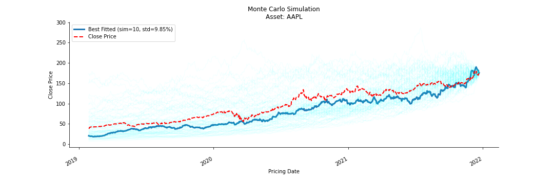
Monte Carlo Simulation is used to evaluate the risk and return value of an investment porfolio of 50 ETFs. First step is to collect historical financial data in 20 years available on fmpcloud. Next step is to forecast future prices with Brownian Emotion. This step is repeated n times with a hope that the more we run, the better outcome we get according to The Law of Large Number. We chose the best model which has the least standard deviation error.

Project description

Data Collection

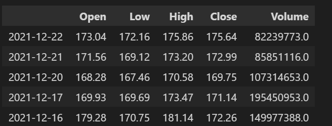
20 years of historial timeseries data is collected from fmpcloud. This site provides a parameterized RESTFul API with 255 free requests. The return object is an array of JSON which contains Close, Adjusted Close, High, Open, Volume of Price Exchange, Pricing Date.

Data Processing

We extract only Close price and price date from raw dataset, convert Date from string to DateTime. The processed data is saved into csv files.

Future Price Simulation with Geometric Brownian Motion

The mathematical expression according to (Making Sense of Monte Carlo):

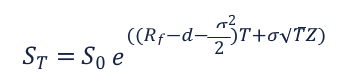
The definitions for each of the variables in this formula are:
- S~T~: Simulated future stock price at the time T.
- S0: Beginning stock price at the time T0
- e: The mathematical constant e (~2.72, i.e., the base of the natural logarithm).
- Rf: The risk-free interest rate based on zero-coupon U.S. Treasuries (the “drift”).
- d: The dividend yield (if applicable). In this case, we work on Close price only and dividend=0.
- σ: Annual volatility.
- T: The term of the award, from the grant date to the end of the applicable period.
- Z: Normally distributed random variable (Z-score); for simplicity, one can think of “Z” as a random number that changes for each simulation.

Implementation

Calculate Asset's Return Values and normalise it with Log

@jit(fastmath=True, forceobj=True)
def f_log_return_value(np_price):
    """Calulate the return value of assets on stock market.
    returns = (price(t) - price(t-1))/price(t-1)
    """
    next_price = np_price[1:]
    # this step is like series.shift(1).iloc[1:]
    next_shift_price = np.append(np.NAN, np_price[:-1])[1:]
    return np.log(next_price/next_shift_price)

Calculate Drift Rate

Drift rate is the risk-free interest rate which is calculated using the standard deviation to measure stock's volatility.

@jit(fastmath=True, forceobj=True)
 def f_get_drift_rate(np_returns):
    """
    Drift rate is the risk-free interest rate. 
    It is calculated using the standard deviation to measure stock's volatility.
    """
    return np.mean(np_returns) - np.var(np_returns)/2

Predict future price with Geometric Brownian Motion

@jit(fastmath=True, forceobj=True)
def f_forecast_price(np_returns, np_drift_rate, current_price):
    """
    Forecast the future prices with Geometric_Brownian_motion.
    The mathematical expression is taken from this article: corpgov.law.harvard.edu/2019/08/18/making-sense-of-monte-carlo/
    """
    # Calculate normally distributed random variable
    zscore =  rd.gauss(0,1)   
    # Calculate stochastic differential equation (SDE)
    np_sde = np_drift_rate + ( np.std(np_returns) * zscore )
    # Calculate simulated future stock price in the the future.
    simulated_price = current_price * np.exp(np_sde)
    return simulated_price

Monte Carlo Simulation

We construct a model to get mean and variance of its residual (return).
We forcast the future price using Geometric Brownian Motion (GBM) with drift rate.
We calculate the output of MC Simulation using GBM with drift rate and determine the best fit along with its standard deviation error.
The pseudo random number is generated via empirical distribution.
We run this simulations as n times. The more , the better according to the Law of Large Numbers
We pick the forecast that has the least standard deviation against the original Close prices

we would check if the best forecast can predict the future direction (instead of actual price) and how well monte - carlo catches black swans

@jit(parallel=True, forceobj=True)
def f_monte_carlo(np_price, simulation):
    prediction = {}
    for c_sim in prange(simulation):
        #we only care about close price, if there has been dividend issued, we use adjusted close price instead
        prediction[c_sim] = f_gbm_simulation(np_price)
    # Determine the best fitted simulation wit minimum standard deviation
    pickers = f_get_best_fit(simulation, prediction, np_price)
    return prediction, pickers

@jit(parallel=True, forceobj=True)
def f_gbm_simulation(np_price):
    """
    Simulate the future prices with Geometric_Brownian_motion (en.wikipedia.org/wiki/Geometric_Brownian_motion)
    """
    np_returns = f_log_return_value(np_price)
    np_drift_rate = f_get_drift_rate(np_returns)

    prediction = []
    prediction.append(np_price[0])
    for idx in prange(len(np_price) - 1):
        simulated_price = f_forecast_price(np_returns, np_drift_rate, prediction[-1])
        prediction.append(simulated_price)
    return prediction

@jit(parallel=True, forceobj=True)
def f_get_best_fit(simulation, prediction, np_price):
    """
    # we use simple criterias, the smallest standard deviation
    # we iterate through every simulation and compare it with actual data
    # The winner is the one with minimum standard deviation.
    """
    std = np.finfo(np.float64).max
    pickers = {}
    for c_sim in prange(simulation):
        temp = np.std(np.subtract(prediction[c_sim], np_price))
        if (std > temp):
            std = temp
            pickers = {c_sim: std}
    return pickers

Running on MeluXina

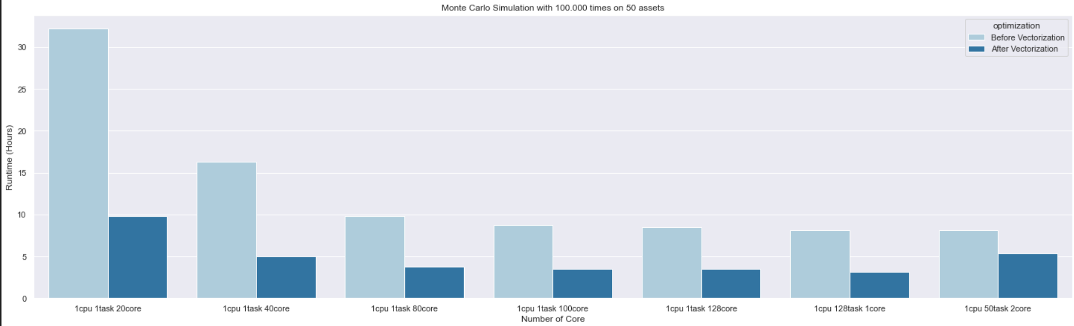
The simulation is run on MeluXina with 1 CPU node, and scaled from 1 to 128 cores in order to measure performance and speedup.

In order to use the computing and memory resources on MeluXina, a slurm job should be created and submitted to the queueing system. Job launcher examples:

#!/bin/bash -l
#SBATCH -A ACCOUNT
#SBATCH --job-name="1cpu"
#SBATCH -N 1
#SBATCH --ntasks=1
#SBATCH --cpus-per-task=128
#SBATCH --output=cpu_scaling.%J.out
#SBATCH --error=cpu_scaling.%J.err
#SBATCH -p cpu
#SBATCH -q default
#SBATCH --time=48:00:00
# Load Python and other needed packages, run code

More details on writing efficient Slurm scripts and scheduling can be found in the Handling jobs section.

Parallelization with Numba

Submitting jobs to a HPC system is just the beginning. The application that will run also needs to be paralelled and vectorized to leverage the HPC power.

In this project, we use Python's concurrent.futures and ProcessPoolExecutor which are high-level interface task distribution to asynchonously schedule and execute tasks on seperated processes. In addition, we use Numba to speed up Python code.

Numba provides a number of compilation options to accelarate the computation. In this project, @jit(nopython=True, parallel=True) and @jit(fastmath=True, forceobj=True) decorators are used to enable automatic iterations and vectorize mathematical calculations. Below are a few examples of how to apply Numba decorators on the code:

Parallelization

@jit(parallel=True, forceobj=True)
def f_get_best_fit(simulation, prediction, np_price):
    """
    # we use simple criterias, the smallest standard deviation
    # we iterate through every simulation and compare it with actual data
    # The winner is the one with minimum standard deviation.
    """
    std = np.finfo(np.float64).max
    pickers = {}
    for c_sim in prange(simulation):
        temp = np.std(np.subtract(prediction[c_sim], np_price))
        if (std > temp):
            std = temp
            pickers = {c_sim: std}
    return pickers

Vectorization

@jit(fastmath=True, forceobj=True)
def f_log_return_value(np_price):
    """Calulate the return value of assets on stock market.
    returns = (price(t) - price(t-1))/price(t-1)
    """
    next_price = np_price[1:]
    # this step is like series.shift(1).iloc[1:]
    next_shift_price = np.append(np.NAN, np_price[:-1])[1:]
    return np.log(next_price/next_shift_price)

Performance Report

The difference between non-vectorization and vectorization executions on MeluXina:

Monte Carlo Simulation

Overview of the showcase

Project description

Data Collection

Data Processing

Future Price Simulation with Geometric Brownian Motion

Implementation

Running on MeluXina

Parallelization with Numba

Performance Report

References