Tutorial: A simple Monte Carlo pi Estimation with Multiprocessing and VizTracer
Introduction
In this tutorial, we'll perform multiple Monte Carlo simulations to approximate Pi using Python's multiprocessing. We'll see how the number of points affects the runtime and use VizTracer for visualizing the execution.
Prerequisites
In the following, we launch an interactive session on a cpu node.
salloc -A [YOUR ACCOUNT] -p cpu --qos default -N 1 -t 8:00:0
we can then install the required packagea for what follows:
python -m pip install --user matplotlib pandas viztracer
Step 1: Writing the Python Code
Create a file demo_viztracer.py and paste the provided code into it:
import os
import pandas as pd
import datetime
import time
# import numexpr as ne
import random
import logging
import numpy as np
logging.getLogger().setLevel(level=logging.DEBUG)
logging.info("Logging set up")
def PI_MC(runNumber, numberOfPoints):
write_process_id_to_process_file('process_list.txt')
inside_circle = 0
start_time = time.time()
for __ in range(numberOfPoints):
x, y = random.random(), random.random()
if x**2 + y**2 <= 1:
inside_circle += 1
ellapsed = time.time() - start_time
pid = os.getpid()
print(f"Process ID: {pid} took {ellapsed} seconds\n")
return runNumber, pid, numberOfPoints, 4 * inside_circle / numberOfPoints, ellapsed
def write_to_process_file(file_path):
with open(file_path, 'w') as file:
current_time = datetime.datetime.now()
pid = os.getpid()
data_to_append = f"Starting main process {current_time}.\n. Master process is {pid}\n"
file.write(data_to_append)
def write_process_id_to_process_file(file_path):
pid = os.getpid()
current_time = datetime.datetime.now()
# Prepare the data to append
data_to_append = f"{current_time} - Process ID: {pid}\n"
file_path = 'process_list.txt'
with open(file_path, 'a') as file:
file.write(data_to_append)
def post_process(df):
import matplotlib.pyplot as plt
# Histogram showing the number of occurrences per processId
plt.figure(figsize=(10, 6))
df['processId'].value_counts().plot(kind='bar')
plt.title('Number of Occurrences per ProcessID')
plt.xlabel('ProcessID')
plt.ylabel('Number of Occurrences')
plt.draw()
plt.savefig('process_id_histogram.png')
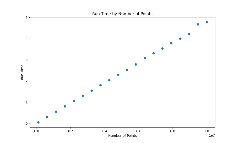
# Scatter plot showing the runtime by number of points
plt.figure(figsize=(10, 6))
plt.scatter(df['numberOfPoints'], df['runTime'])
plt.title('Run Time by Number of Points')
plt.xlabel('Number of Points')
plt.ylabel('Run Time')
plt.draw()
plt.savefig('run_time_scatter.png')
df['error'] = np.abs(df['result'] - np.pi)
plt.figure(figsize=(10, 6))
plt.scatter(df['numberOfPoints'], df['error'])
plt.title('Run Time by Number of Points')
plt.xlabel('Number of Points')
plt.ylabel('Run Time')
plt.draw()
plt.savefig('error_scatter.png')
plt.figure(figsize=(10, 6))
# Grouping by 'processId' and summing 'runTime'
grouped_data = df.groupby('processId')['runTime'].sum()
# Plotting the histogram
grouped_data.plot(kind='bar')
plt.title('Sum of runTime Grouped by processId')
plt.xlabel('Process ID')
plt.ylabel('Total runTime')
plt.draw()
plt.savefig('runTimeByProcess.png')
def run_loop():
import concurrent.futures
nEstimations = 20
minNPoints = 1e5
maxNPoints = 1e7
params = [(runNumber, nPoints) for runNumber, nPoints in enumerate(np.linspace(minNPoints, maxNPoints, nEstimations).astype(int)) ]
with concurrent.futures.ProcessPoolExecutor(max_workers=3) as executor:
# Submit the function to the executor
futures = [executor.submit(PI_MC, *p) for p in params]
# Retrieve and process the results as they complete
results = []
for future in concurrent.futures.as_completed(futures):
results.append(future.result())
return results
if __name__ == "__main__":
import argparse
parser = argparse.ArgumentParser(description="The script expects either --run or --postprocess.")
group = parser.add_mutually_exclusive_group(required=True)
group.add_argument('--run', action='store_true', help='Run the main process')
group.add_argument('--postprocess', action='store_true', help='Run the postprocessing')
args = parser.parse_args()
file_path = 'MC_PI.h5'
data_key = 'my_dataset'
if args.run:
write_to_process_file('process_list.txt')
results = run_loop()
df = pd.DataFrame(results, columns=['runNumber', 'processId', 'numberOfPoints', 'result', 'runTime'])
# Save DataFrame to HDF5 file
df.to_hdf(file_path, key=data_key)
elif args.postprocess:
df = pd.read_hdf(file_path, key=data_key)
post_process(df)
This script includes in particular:
PI_MC: Function that performs the Monte Carlo simulation.run_loop: Function to manage the multiprocessing pool.
Step 2: Running the Code with VizTracer
Running the code
If you just want to run the code:
python demo_viztracer.py --run
If you want to visualize the multiprocessing behavior, use the following:
python -m viztracer --ignore_c_function --ignore_frozen --log_func_exec='run_loop' -- demo_viztracer.py --run
This command will generate a results.json file with the profiling data.
Note that the option --log_func_exec='run_loop' allows to only trace the function of interest.
Getting the matplotlib figures
After having run the code at least once with one of the two options above, run:
python demo_viztracer.py --postprocess
Step 3: Analyzing the Results
Matplotlib is used to create plots that we can see hereafter.
Fig1: The absolute error of the estimation of pi over the number of points
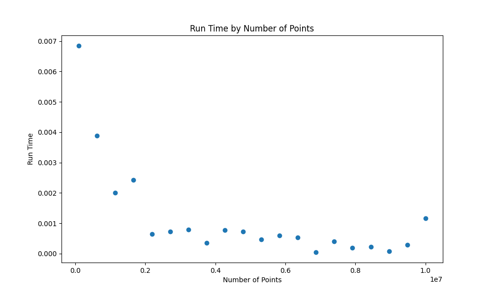
Fig2: Distribution of tasks among processes
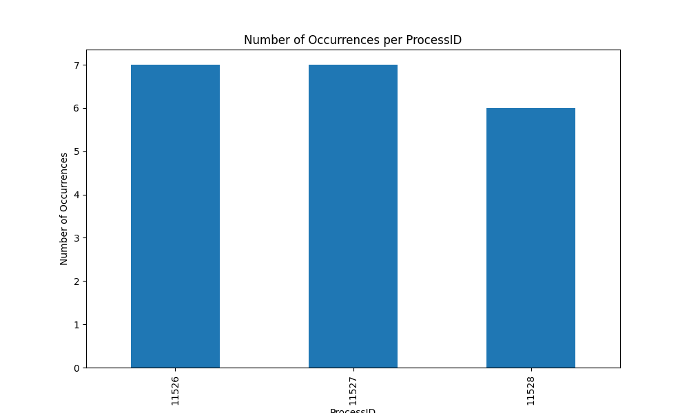
Fig3: Distribution of the runtime among processes
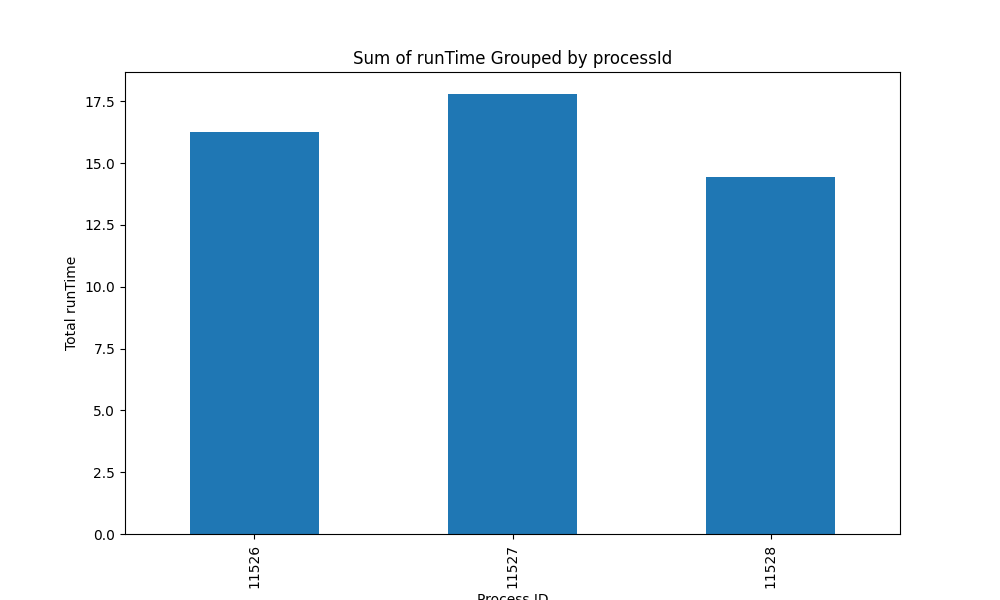
Fig4: Individual task runtime
Step 4: Visualizing Process Execution
We will now use vizviewer to look at what happened at the process level. To use vizviewer, you can set up a port forwarding or an sshfs session in order to be able to have the GUI of vizviewer displayed.
$ vizviewer result.json
Running vizviewer
You can also view your trace on http://localhost:9001
Press Ctrl+C to quit
vizviewer results.json
Let's quickly dig into the output and use the process_list file which was generated at runtime
$ cat process_list.txt
Starting main process 2024-02-23 15:17:24.859507.
. Master process is 11445
2024-02-23 15:17:24.884173 - Process ID: 11526
2024-02-23 15:17:24.884385 - Process ID: 11527
2024-02-23 15:17:24.884488 - Process ID: 11528
2024-02-23 15:17:24.933217 - Process ID: 11526
2024-02-23 15:17:25.182257 - Process ID: 11527
2024-02-23 15:17:25.434973 - Process ID: 11528
...
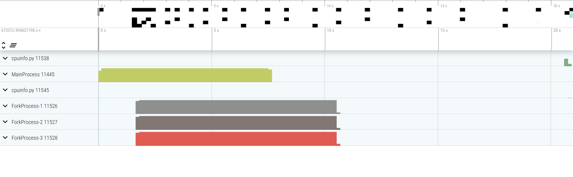
It looks like 11445 is the master process and the 3 workers are 11526, 11527 and 11528.
This is also what we see with vizviewer:
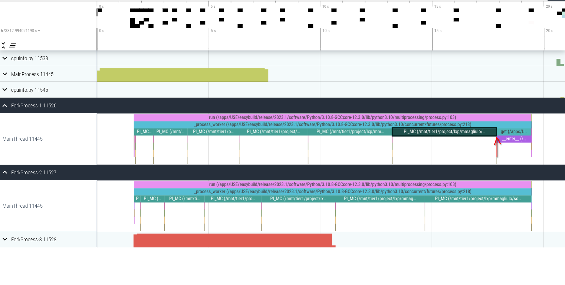
Now if we look at the workers, we can see interesting things:
- the function
PI_MCtakes more and more time as the number of sample points increases (makes sense :p) - the process 11526 finishes to work earlier than 11527 and stays idle until the completion of the pool of processes. This confirms what we saw in Figure 2!
Conclusion
This tutorial demonstrates using Python's multiprocessing for a computationally intensive Monte Carlo simulation. The VizTracer tool provides insights into how tasks are distributed and executed by different processes.